Benchmarking Keras Core: A Comparative Analysis with TensorFlow Keras on CIFAR-10 using Google Colab A100 GPU

In the diverse world of deep learning frameworks, making an informed choice often resembles navigating through a dense forest with a compass that has a penchant for dramatic mood swings. Among the torchbearers leading the way, a new entrant, Keras Core, emerges as a contender worthy of the spotlight. This nascent evolution of the original Keras library is stirring up the waters with its promise of a streamlined, user-friendly interface while still retaining the charm and efficiency that made Keras a beloved tool among machine learning practitioners. The exciting news around its development has the community buzzing with anticipation, as Keras Core is poised to not only carry the legacy of Keras but propel it into a new era of deep learning innovation.

As we venture into this jungle with a benchmarking machete, our objective is simple yet profound - to dissect the performance of Keras Core as compared to the mature TensorFlow framework on the vivacious CIFAR-10 dataset, under the spotlight of Google Colab’s A100 GPU.

Now, why benchmark, you may ask? Benchmarking is akin to the reality TV show of the deep learning realm. It strips down the contenders to their core, exposing the raw performance that lurks beneath the polished APIs. It provides a data-driven stage for frameworks to strut their stuff, showcasing how they fare in memory consumption, training speed, and accuracy, among other thrilling episodes of the deep learning saga.

So tighten your seat belts- I meant GPUs!!

The Ingredients of Benchmarking Feast

Before diving into the depths of our benchmarking experiment, let’s familiarize ourselves with the key players that will be centre stage in this performance:

• Keras Core: An exhilarating evolution of the original Keras library, Keras Core bursts onto the scene with the promise of streamlined, user-friendly interfaces for crafting and training deep learning models. But here's where it gets thrilling - Keras Core comes with a multi-backend charm! That's right, at the onset of your deep learning adventure, you get to choose whether to team up with TensorFlow, join forces with PyTorch, or ally with JAX. This capability to choose your backend before diving into the model-building arena is what makes Keras Core a fascinating new player on the field, and we're all eyes to see how it fares against the seasoned TensorFlow framework in our benchmarking showdown.
• TensorFlow: A veteran in the field, TensorFlow is a comprehensive, open-source machine learning framework with a vast community and ecosystem. Its high-performance capabilities for large-scale machine-learning tasks make it a benchmarking favourite.
• Google Colab’s A100 GPU: A powerhouse of computation, the A100 GPU on Google Colab provides the muscle needed for heavy lifting in our benchmarking experiment. Its robust architecture allows for speedy training and inference, making it a choice platform for comparing framework performance.
• CIFAR-10 Dataset: The CIFAR-10 dataset, with its modest size yet challenging image classification task, serves as the proving ground for our frameworks. Consisting of 60,000 32x32 colour images across 10 classes, it provides a balanced playground to evaluate the models' performance.
• LeNet Architecture: A classic yet evergreen architecture in the realm of Convolutional Neural Networks (CNNs), LeNet stands tall as a testament to the fundamental principles of deep learning. Pioneered by Yann LeCun and his team during the '90s, LeNet's structured layers of convolution, pooling, and fully connected nodes have inspired a multitude of modern architectures. Its simplistic yet effective design makes it an ideal candidate for our benchmarking endeavour, providing a common ground to evaluate the prowess of TensorFlow and Keras Core in a head-to-head match-up. Whether it's TensorFlow's seasoned stability or Keras Core's fresh vigour, LeNet's architecture will ensure they both get a fair arena to exhibit their mettle.

Unsheathing the Coding Sword: The Benchmarking Odyssey Begins

In this section, we roll up our sleeves, unsheathe the coding sword, and delve into the heart of the benchmarking odyssey. Armed with the potent blend of TensorFlow, Keras Core, and the LeNet architecture, our quest for unveiling the quintessence of performance begins. So, let's draw the first line of code and embark on this enlightening journey!
Before our code gladiators step into the arena, it's imperative to ensure a level playing field. Reproducibility is our guiding star, and setting seeds is our homage to it. This modest yet crucial step ensures that the randomness inherent in our training process remains consistent, paving the way for a fair comparison. Now, let us delve into crafting a function capable of building the LeNet model. To uphold the banner of reproducibility, we are explicitly initializing the weights and biases using the Glorot Uniform initialization. Additionally, to keep tabs on the memory footprint during this showdown, we're enlisting the aid of 'psutil'. Without further ado, here is the function:

def create_lenet(keras, input_shape=(32, 32, 3), num_classes=10):
  """
  Creates a LeNet model using the specified Keras library.


  Parameters:
  - keras (module): The Keras library (either tensorflow.keras or keras_core).
  - input_shape (tuple): The shape of the input images.
  - num_classes (int): The number of output classes.


  Returns:
  - model (keras.Model): The constructed LeNet model.
  """
  # Measure memory usage before creating the model
  memory_before = psutil.virtual_memory().used
  initializer = keras.initializers.GlorotUniform(seed=0)
  model = keras.models.Sequential()
  # Layer 1: Convolutional Layer with  Glorot Uniform initialization
  model.add(keras.layers.Conv2D(filters=6, kernel_size=(5, 5), strides=(1, 1),
  activation='tanh', input_shape=input_shape,
  kernel_initializer=initializer, bias_initializer=initializer))
  # Layer 2: Average Pooling Layer
  model.add(keras.layers.AveragePooling2D(pool_size=(2, 2), strides=(2, 2)))
  # Layer 3: Convolutional Layer with  Glorot Uniform initialization
  model.add(keras.layers.Conv2D(filters=16, kernel_size=(5, 5), strides=(1, 1),
  activation='tanh',
  kernel_initializer=initializer, bias_initializer=initializer))
  # Layer 4: Average Pooling Layer
  model.add(keras.layers.AveragePooling2D(pool_size=(2, 2), strides=(2, 2)))
  # Flatten the output to feed it into Dense Layers
  model.add(keras.layers.Flatten())
  # Layer 5: Fully Connected Layer with  Glorot Uniform initialization
  model.add(keras.layers.Dense(units=120, activation='tanh',
  kernel_initializer=initializer, bias_initializer=initializer))
  # Layer 6: Fully Connected Layer with  Glorot Uniform initialization
  model.add(keras.layers.Dense(units=84, activation='tanh',
  kernel_initializer=initializer, bias_initializer=initializer))
  # Layer 7: Output Layer with  Glorot Uniform initialization
  model.add(keras.layers.Dense(units=num_classes, activation='softmax',
  kernel_initializer=initializer, bias_initializer=initializer))
  # Measure memory usage after creating the model
  memory_after = psutil.virtual_memory().used

  # Calculate the increase in memory usage
  memory_increase = (memory_after - memory_before) / (2**20) # Convert bytes to MiB
  print(f'Memory increase: {memory_increase:.2f} MiB')
  return model

As we descend further into the heart of our benchmarking expedition, we now arm ourselves with three trusty companions - a trio of functions, each with its unique prowess. Let's unveil our code warriors:

First, we introduce `train_model`, our diligent trainer. With a keen eye on the clock and a vigilant watch over memory usage, it guides our model through the grueling regimen of training epochs, all while keeping a meticulous log of the time and memory spent in honing the model to perfection.

def train_model(model, data, labels, epochs=10):
  start_time = time.time() # Record start time
  mem_usage_before = psutil.virtual_memory().used
  history = model.fit(data, labels, epochs=epochs)
  mem_usage_after = psutil.virtual_memory().used
  end_time = time.time() # Record end time
  # Calculate and print the training time
  training_time = end_time - start_time
  print(f'Training time: {training_time} seconds')
  mem_increase = (mem_usage_after - mem_usage_before) / (2**20)
  print(f'Increase in memory during training: {mem_increase:.2f} MiB')
  return history

Next, in the spotlight is `benchmark_inference`, our swift scout. With a knack for speed, it races through the data, making inference a breeze. It’s all about timing the sprint right, as it dashes through the dataset, recording the time it takes for our model to make predictions.

def benchmark_inference(model, data):
  start_time = time.time()
  predictions = model.predict(data)
  end_time = time.time()
  inference_time = end_time - start_time
  print(f'Inference time for {len(data)} samples: {inference_time} seconds')

Last but not least, we have `benchmark_performance`, our astute analyst. It dives into the depths of performance metrics, resurfacing with treasured insights into the model's accuracy, precision, recall, and F1 score on the battlefield of data. A data-driven sage, it lays out a detailed account of how our model fared, presenting a tableau of performance metrics that tell tales of our model's valour.

def benchmark_performance(model, data, labels, dataset_name):
  # Predict the labels
  predictions = model.predict(data)
  predicted_classes = np.argmax(predictions, axis=1)


  # If the labels are one-hot encoded, convert them to class indices
  if labels.ndim > 1:
  labels = np.argmax(labels, axis=1)


  # Compute the metrics
  accuracy = accuracy_score(labels, predicted_classes)
  f1 = f1_score(labels, predicted_classes, average='weighted')
  precision = precision_score(labels, predicted_classes, average='weighted')
  recall = recall_score(labels, predicted_classes, average='weighted')


  # Create a DataFrame to hold the metrics
  metrics_df = pd.DataFrame({
  'Dataset': [dataset_name],
  'Accuracy': [accuracy],
  'F1 Score': [f1],
  'Precision': [precision],
  'Recall': [recall]
  })


  return metrics_df

Armed with our craftily coded functions, it's time to conjure up the LeNet models from the digital ether. With a flourish of our coding wand, we invoke the create_lenet spell twice, once with the essence of TensorFlow Keras and once with the spirit of Keras Core

lenet_model_tf_keras = create_lenet(tf_keras)


lenet_model_core_keras = create_lenet(core_keras)

Take a look at the structure of our freshly created LeNet models. Not only do we see their detailed layers, but we also highlight how much memory they use. The TensorFlow Keras model needs about 668 MiB of memory, while the Keras Core model is much more memory-efficient, using 729 MiB.

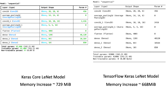
The negligible gap in memory consumption underscores each model's adeptness at resource allocation—a critical factor that might influence their overall performance. With the preliminaries out of the way, it’s time to thrust these models into the arena and witness the spectacle of their computational prowess.

Training Time and Memory Requirements

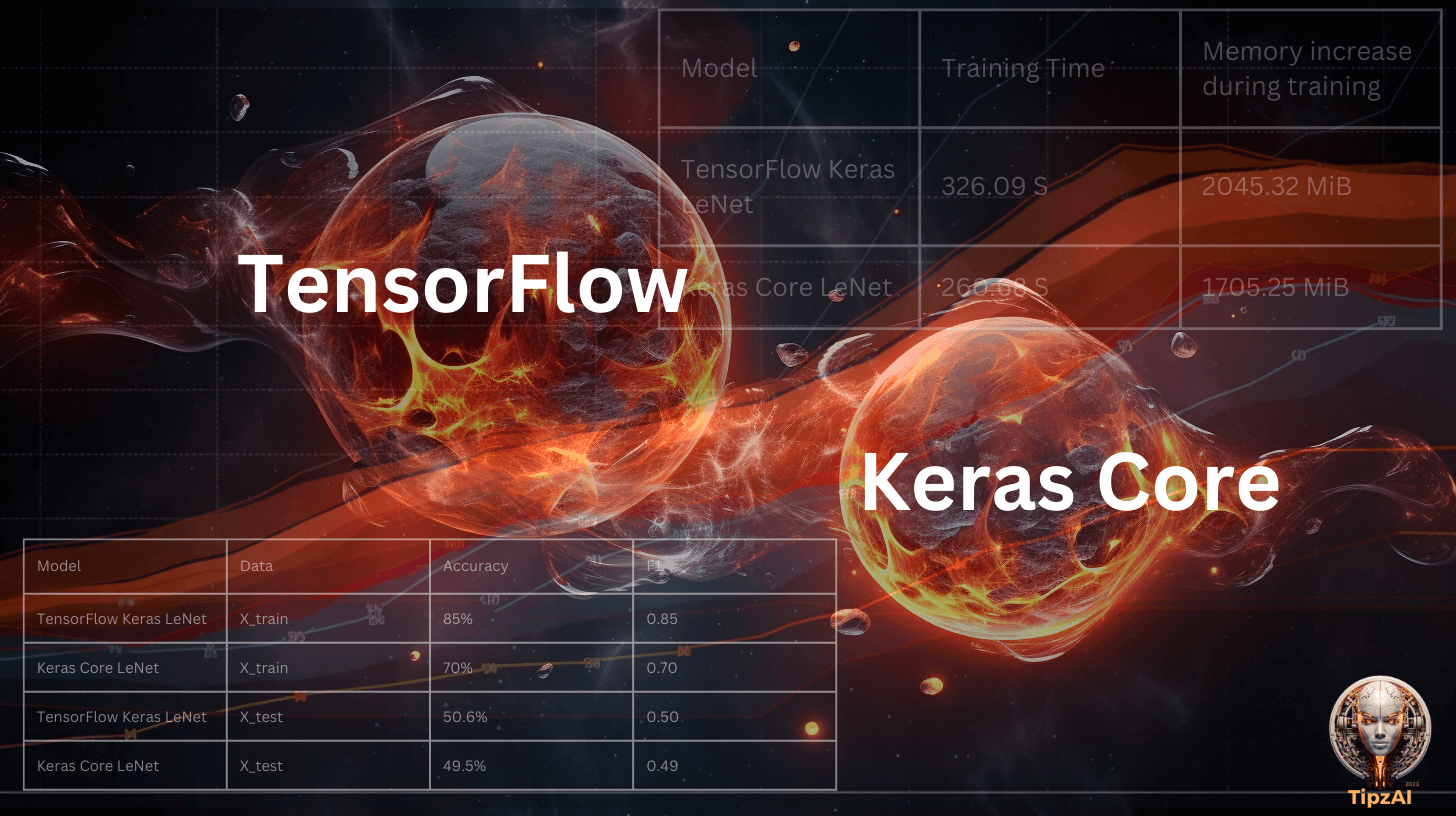
Next, moving towards training, the two models, the table below summarises the training time and memory used while training:

Each number in our table tells a story of efficiency and capability. The 'Training Time' represents the speed at which our models can learn from the data. A lower training time means a quicker turnaround from data to deployment, which is crucial in dynamic environments where models need to be updated or retrained frequently.

The 'Memory Increase During Training' reflects the additional memory required by the model during the learning process. In contexts where resources are limited, such as on-edge devices or in production environments with strict memory constraints, a lower memory footprint is highly desirable. It indicates a model that is not just faster to train but also leaner in its resource consumption, making it ideal for scenarios where efficiency is paramount.

The Keras Core model is not just faster but also more memory-efficient. This makes it a strong candidate for environments where both time and memory resources are at a premium.

The tale of the tape in our benchmarking showdown between TensorFlow Keras and Keras Core models provides insights into their learning efficacy and generalization capabilities.

The TensorFlow Keras LeNet model boasts an impressive accuracy of 85% and an F1 score of 0.85, showcasing robust learning from the training data. In contrast, the Keras Core LeNet model trails with a 70% accuracy and an F1 score of 0.70, hinting at room for improvement in its learning strategy.

Upon evaluation with the test dataset, the TensorFlow Keras LeNet model secured a moderate accuracy of 50.6% and an F1 score of 0.50. The Keras Core model performed similarly, with a close accuracy of 49.5% and an F1 score of 0.49. This performance dip on unseen data suggests overfitting—a hurdle often encountered in machine learning models, particularly when navigating the complexities of a dataset like CIFAR-10.

While the conversation on mitigating overfitting is extensive and reserved for another occasion, it's noteworthy that the real crucible for these models is their prowess on unfamiliar data. Here, our two contenders are virtually in a dead heat, underscoring the competitive edge of TensorFlow Keras in learning, albeit by a slender margin

And the verdict!

In the final reckoning of our benchmarking endeavour, Keras Core has showcased its potential as an emerging contender, demonstrating commendable performance and efficiency. While TensorFlow Keras maintains a slight edge in accuracy and learning capability, Keras Core's competitive training time and memory usage highlight its growing stature and optimization.

For practitioners and researchers, the choice between Keras Core and TensorFlow Keras may ultimately hinge on specific project needs and resource constraints. TensorFlow Keras remains the go-to for those seeking established stability and performance. In contrast, Keras Core represents a promising alternative, particularly appealing for environments where agility and a lighter memory footprint are at a premium.